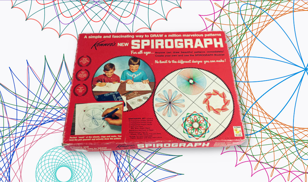
A Spirograph is worth a thousand words
I used to love playing with these things as a kid. If you aren’t familiar, Spirograph is basically an art kit that lets you draw cool spiral shapes. Below is a demonstration from one of their commercials.
I had the idea to recreate these designs with Python and Matplotlib. There’s a bit of math involved but it’s not as complicated as you might think. We’ll skip the odd shapes like ovals and triangles and stick with basic circles for now.
1. Math.
To understand what’s happening, it helps to start with cycloid curves. Forget spirographs for a moment and imagine a point on the edge of a rolling wheel. The path traced by that point is called a cycloid.
We can predict the point’s position (x, y) as a function of angular rotation (t) using a pair of parametric equations.

Note: Naming the independent variable t is a convention in parametric equations. It doesn’t generally represent time. But in this case, if you assume the speed of angular rotation is constant, you can think of position as a function of time.
Imagine dragging a pen around that point on the edge of the circle. You could create fun designs! That’s what we’re attempting to do here.
But first we have to move from a flat surface to the inside a large circle. The path traced in that case is called a hypocycloid.
Its equations are a little more complicated but still not outrageous.

Where…
- R is the radius of the large circle.
- r is the radius of the small circle.
- L is the length from the small circle’s center to the pen.
- ρ (“rho”) is the ratio of L to r.
Technically the traced path is called a hypotrochoid. A hypocycloid is a special case where the pen (the red dot) is on the edge of the small circle and R is a multiple of r. I don’t expect anyone outside university math departments to care, but Spirographs make more sense if we start by considering the special case—the hypocycloid.
2. Code.
We’ll create an animated GIF that shows a pen tracing a hypocycloid curve. The script will start at t=0.0 and a large for loop will increment t while saving images.
First define constants. Let’s follow the diagram above and make R four times the size of r. So if we wanted to, we could line up four small circles within the large one.
rho defines how far from the small circle’s center the pen is held. Setting it to 1.0 means the pen is on the outer edge, which is what we want.
The GIF will animate one full 360° trip around the large circle. When the script finishes running, t will equal 2π. t_steps is the number of frames generated throughout that motion.
R = 4
r = 1
rho = 1.0
t_steps = 300
Begin by setting t=0.0. In our equations, the small circle starts at zero degrees—to the east of the origin.
Since we’re drawing the pen’s path as it’s created, we need to record a history of every position it’s been up to the current moment. Then we’ll be able to call plot() and pass the two movement_history lists.
Remember that t_steps defines how many frames are generated, i.e. the number of passes through the for loop. Name the loop variable frame_counter and we can use it when saving images.
import matplotlib.pyplot as plt

t = 0.0

movement_history_x = []
movement_history_y = []

plt.style.use("wollen_spirograph.mplstyle")

for frame_counter in range(t_steps):
    print(f"{frame_counter + 1}/{t_steps}")

    fig, ax = plt.subplots()

    [...]
Let’s draw a “crosshair” through axes lines. That should help the viewer’s eyes to judge the small circle’s location.
Draw circles using Matplotlib patches. You could obviously generate points manually but it’s easier to define a circle’s center point and radius and let Matplotlib take care of it.
No matter where the small circle is located, its center point will always be a fixed distance from the large circle’s center (R – r).
from math import sin, cos, pi
from matplotlib.patches import Circle

for frame_counter in range(t_steps):

    [...]

    # Axis Lines:
    ax.plot([-R * 10, R * 10], [0, 0], c="#888", lw=1.0, zorder=1)
    ax.plot([0, 0], [-R * 10, R * 10], c="#888", lw=1.0, zorder=1)

    # Big Circle:
    ax.add_patch(Circle((0, 0), R, fc="None", ec="#000", lw=1.5, zorder=3))

    # Small Circle:
    center_point_x = (R - r) * cos(t)
    center_point_y = (R - r) * sin(t)
    ax.scatter([center_point_x], [center_point_y], c="#000", s=20, zorder=3)
    ax.add_patch(Circle((center_point_x, center_point_y), r, fc="None", ec="#000", lw=1.5, zorder=3))

    [...]
Now we can draw the little red dot that represents the pen. Its (x, y) position is given by the equations above. Implement the equations using sin and cos from the math library.
Plot the pen tip using scatter and remember to append its (x, y) coordinates to their respective movement history lists.
Then call plot to draw a line tracing all those points up to the current moment. Let’s do a red dashed line to ensure it stands out.
for frame_counter in range(t_steps):

    [...]

    # Ball Point Pen:
    pen_point_x = (R - r) * cos(t) + rho * r * cos((R - r) / r * t)
    pen_point_y = (R - r) * sin(t) - rho * r * sin((R - r) / r * t)
    ax.scatter([pen_point_x], [pen_point_y], c="#F00", s=40, zorder=4)
    movement_history_x.append(pen_point_x)
    movement_history_y.append(pen_point_y)
    ax.plot(movement_history_x, movement_history_y, c="#F00", ls="--", lw=1.0, zorder=2)

    [...]
It’s a good idea to define ticks and window limits as a function of R, the big circle’s radius. That will make it easy to adjust constants at the top of the page.
for frame_counter in range(t_steps):

    [...]

    ticks = range(-R, R + 1)
    ax.set(xticks=ticks,
           yticks=ticks,
           xlim=(-R * 1.05, R * 1.05),
           ylim=(-R * 1.05, R * 1.05))

    [...]
Make a note of those constants in the top-right corner with text. It will make it clear exactly what parameters were used in generating the animation.
for frame_counter in range(t_steps):

    [...]

    ax.text(x=R * 0.99,
            y=R * 0.98,
            s=f"R = {R:.1f}\nr = {r:.1f}\nρ = {rho:.1f}",
            ha="right",
            va="top")

    [...]
Finally, save and close the figure, which will prevent Matplotlib from holding every frame in memory.
Remember to increment t. We know t counts up to 2π and we know it takes t_steps frames to get there.
for frame_counter in range(t_steps):

    [...]

    plt.savefig(f"frames/{frame_counter}.png")

    plt.close()

    t += 2 * pi / t_steps
After running the script, you’ll have 300 images in a frames folder. There are many options to convert PNG files into an animated GIF. The image editor GIMP is one of the easiest. I’ve gotten used to FFMPEG, a command-line tool.
3. The output.
Since the small circle’s diameter is 1/4 of the large circle, it does exactly four rotations during its trip. The resulting diamond shape is called an astroid. You can change the ratio and create all sorts of hypocycloid curves.
But it gets more interesting when the R/r ratio isn’t a nice even number. What if the small radius is 1.63? Then the path won’t close neatly after a single 360° trip. It will be shifted slightly over and repeat itself, which is how those cool Spirograph designs emerge.
We also don’t have to keep the pen at the outer edge of the small circle. Change rho to 0.47 and it will be about halfway between the small circle’s center point and its edge.
I plotted four Spirograph designs that I thought were interesting. I won’t post the code but it’s essentially the same as above, except with tweaks to R, r, and rho as described. t is scaled to allow for three full trips around the large circle.

This GIF is hypnotizing to me. Small adjustments to the parameters lead to wildly different designs. You could change color and line width for even more customization, like swapping out your pen in real life.
Download the Matplotlib style.
Full code:
from math import sin, cos, pi
import matplotlib.pyplot as plt
from matplotlib.patches import Circle


R = 4
r = 1
rho = 1.0
t_steps = 300

t = 0.0

movement_history_x = []
movement_history_y = []

plt.style.use("wollen_spirograph.mplstyle")

for frame_counter in range(t_steps):
    print(f"{frame_counter + 1}/{t_steps}")

    fig, ax = plt.subplots()

    # Axis Lines:
    ax.plot([-R * 10, R * 10], [0, 0], c="#888", lw=1.0, zorder=1)
    ax.plot([0, 0], [-R * 10, R * 10], c="#888", lw=1.0, zorder=1)

    # Big Circle:
    ax.add_patch(Circle((0, 0), R, fc="None", ec="#000", lw=1.5, zorder=3))

    # Small Circle:
    center_point_x = (R - r) * cos(t)
    center_point_y = (R - r) * sin(t)
    ax.scatter([center_point_x], [center_point_y], c="#000", s=20, zorder=3)
    ax.add_patch(Circle((center_point_x, center_point_y), r, fc="None", ec="#000", lw=1.5, zorder=3))

    # Ball Point Pen:
    pen_point_x = (R - r) * cos(t) + rho * r * cos((R - r) / r * t)
    pen_point_y = (R - r) * sin(t) - rho * r * sin((R - r) / r * t)
    ax.scatter([pen_point_x], [pen_point_y], c="#F00", s=40, zorder=4)
    movement_history_x.append(pen_point_x)
    movement_history_y.append(pen_point_y)
    ax.plot(movement_history_x, movement_history_y, c="#F00", ls="--", lw=1.0, zorder=2)

    ticks = range(-R, R + 1)
    ax.set(xticks=ticks,
           yticks=ticks,
           xlim=(-R * 1.05, R * 1.05),
           ylim=(-R * 1.05, R * 1.05))

    ax.text(x=R * 0.99,
            y=R * 0.98,
            s=f"R = {R:.1f}\nr = {r:.1f}\nρ = {rho:.1f}",
            ha="right",
            va="top")

    plt.savefig(f"frames/{frame_counter}.png")

    plt.close()

    t += 2 * pi / t_steps