
The golden age of kicking
You might have seen Cam Little’s NFL-record 68-yard field goal last November. It seems like every few weeks there’s a new guy on the scene looking like the greatest kicker of all time.
My theory is that we’re currently in a fleeting golden age of NFL field goal kicking. And like an old-fashioned fable, kickers’ success will beget their downfall. The league will soon rebalance their rules to limit kickers’ effectiveness.
Why would the NFL want to slow them down? It’s a fair question. They have made a lot of changes in recent years to encourage scoring. But with touchbacks now spotting the ball at the 35 yard line and midfield marking the edge of field goal range, it’s become a little too easy to put together a quick scoring drive. I think it’s embarrassing for the league when points come off 15 or 20 yards of offense and a kick—especially because those drives tend to happen late in the 4th quarter in high-stakes moments which are then shared on social media with millions of additional eyeballs. I predict that ultimately the NFL will prefer slightly less scoring to being public embarrassed.
How might they nerf field goals? A few ideas…
- Easiest: Change kicking balls. Either force kickers to use the same ball as the offense or increase kicking balls’ air pressure. This would have the advantage of hiding the rule change from casual viewers.
- Maybe: On the other hand, narrowing field goal uprights or raising the crossbar would be visually obvious and draw a lot of attention.
- Least likely: Give kickers fewer opportunities. Change kickoff/touchback rules and move starting field position further back. I would be surprised if they went this route after putting so much effort into encouraging kick returns. That phase of special teams is genuinely more exciting than it was a few years ago.
Admittedly, this is all idle speculation. Let’s go back to the beginning and verify that NFL kickers are, at least in terms of top-end range, getting significantly better.
1. Acquire the data.
We can start with the Wikipedia page for longest NFL field goals. It lists all 60+ yard performances since the merger. On the blog I usually work with a clean dataset and gloss over the (often tedious) details of where the data came from. Since scraping Wikipedia is relatively easy, let’s step through it.
Disclaimer: the web page may change in the future and break this code!
The data is organized in tables, which is ideal because pandas’ read_html method is very good at pulling HTML tables into a DataFrame.
We catch another break as the tables are not loaded dynamically with Javascript. They render the old-fashioned way with HTML. Therefore we can use Python’s straightforward requests library to download the page.
Wikipedia doesn’t mind scraping as long as we’re respectful and identify ourselves in headers. Today let’s be KickerBot 1.0.
import requests

url = "https://en.wikipedia.org/wiki/List_of_longest_NFL_field_goals"

headers = {"User-Agent": "KickerBot/1.0"}

text = requests.get(url, headers=headers).text

with open("response.txt", "w") as f:
    f.write(text)
It’s important to save the response locally and avoid sending repeated HTTP requests. If you were doing this for real you would need to run the script several times to get everything working correctly. Just comment out the request and file write once the page is saved to disk.
Open the file and feed it into pandas.read_html. Pandas expects a StringIO type rather than a plain string. It then returns a list of DataFrames. Easy, right?
import pandas as pd

with open("response.txt", "r") as f:
    text = f.read()

dfs_found = pd.read_html(StringIO(text))
If you check len(dfs_found) you’ll see we extracted 13 DataFrames. The main table that we want is at the top of the web page so unsurprisingly it’s the first element of the list, i.e. dfs_found[0].
dfs_found[0].head() is shown below:
   Distance            Kicker  ...            Elevation                  Weather
0  68 yards        Cam Little  ...  2,184 ft (666 m)[7]                     Dome
1  67 yards        Cam Little  ...         4 ft (1.2 m)            58 °F (14 °C)
2  66 yards     Justin Tucker  ...    601 ft (183 m)[9]                     Dome
3  65 yards    Brandon Aubrey  ...       584 ft (179 m)  Retractable roof closed
4  65 yards  Chase McLaughlin  ...         35 ft (11 m)            93 °F (34 °C)
We still have a little work to do. Distance column values are string types. We need to strip out the “yards” text and convert to integers. We can drop most of the columns as their information is irrelevant.
Assign this first-element DataFrame to its own variable, df, and limit it to the three relevant columns. It’s good practice to copy the sliced DataFrame before operating further. If you don’t, Pandas will let you know.
df = dfs_found[0][['Distance', 'Date', 'Kicker']].copy()

print(df.head())
The output:
   Distance                Date            Kicker
0  68 yards    November 2, 2025        Cam Little
1  67 yards     January 4, 2026        Cam Little
2  66 yards  September 26, 2021     Justin Tucker
3  65 yards  September 22, 2024    Brandon Aubrey
4  65 yards  September 28, 2025  Chase McLaughlin
That’s a little better. Now we can see that Date is a string type as well. Let’s convert it to datetime while also parsing the Distance column.
The pandas str accessor allows us to use most string methods from base Python.
df['Date'] = pd.to_datetime(df['Date'])

df['Distance'] = df['Distance'].str.strip(" yards").astype(int)

print(df.head())
The output:
   Distance       Date            Kicker
0        68 2025-11-02        Cam Little
1        67 2026-01-04        Cam Little
2        66 2021-09-26     Justin Tucker
3        65 2024-09-22    Brandon Aubrey
4        65 2025-09-28  Chase McLaughlin
We’ve successfully scraped everything we need! Technically we don’t need kickers’ names but it feels wrong to erase them.
Save the DataFrame to a CSV file. Set index=False to exclude the useless index column.
df.to_csv("nfl_fgs_2026-09-03.csv", index=False)
2. Prepare the data.
Read the dataset into a pandas DataFrame. We’ll be using a datetime x-axis so make sure the Date column is the correct type.
df = pd.read_csv("nfl_fgs_2026-09-03.csv", parse_dates=['Date'])
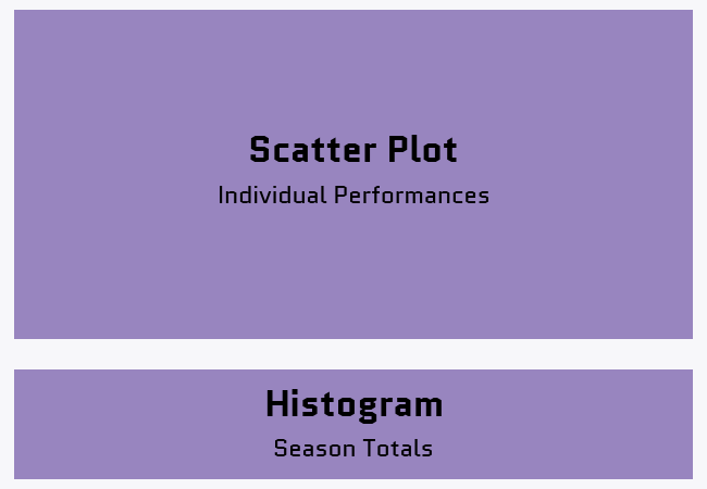
The plan is to create two vertically stacked subplots like below. On top will be a scatter plot of individual field goals. On bottom a histogram, which is essentially a bar plot displaying the total number of 60+ yard field goals per season.
I always try to match x-axes between vertically stacked subplots. It’s important for readability at first glance. In this case it’s not really possible because the scatter plot will use datetimes while the histogram will use annual integers.
To resolve this, let’s treat the histogram x-axis like a datetime axis but locate every bar on January 1st. That way we can easily align the two x-axes.
NFL seasons extend into January and February so, for example, the 2010 season includes dates in January 2011. We can solve this by subtracting 90 days from every date and checking the resulting year. Do this operation and generate a Season column.
df['Season'] = (df['Date'] - pd.Timedelta("90 days")).dt.strftime("%Y").astype(int)
We have an integer Season column but we want bars on January 1st of each year. Use the Season column to create a datetime Season_x column. This is what we’ll use for plotting.
df['Season_x'] = df['Season'].apply(lambda x: pd.Timestamp(f"January 1 {x}"))
df.head() looks like this:
   Distance       Date            Kicker  Season   Season_x
0        68 2025-11-02        Cam Little    2025 2025-01-01
1        67 2026-01-04        Cam Little    2025 2025-01-01
2        66 2021-09-26     Justin Tucker    2021 2021-01-01
3        65 2024-09-22    Brandon Aubrey    2024 2024-01-01
4        65 2025-09-28  Chase McLaughlin    2025 2025-01-01
That looks great. Now we need to groupby season and count how many rows exist per year. The reset_index() addition isn’t required but it will make addressing columns a little more intuitive.
df2 = df.groupby("Season_x")['Distance'].agg("count").reset_index()

print(df2.tail())
The new DataFrame is below. You could rename “Distance” to “count” or similar but this will suffice.
     Season_x  Distance
16 2021-01-01         3
17 2022-01-01         5
18 2023-01-01         4
19 2024-01-01         4
20 2025-01-01        12
We’ll use df2 to build our histogram. Bars will be located at January 1st of each year and the corresponding value will be their height.
3. Plot the data.
I’ll use a custom Matplotlib style that will be linked at the bottom of this post.
Create a 2×1 subplot grid and specify height_ratios so the lower histogram is smaller. We can refer to the Axes as ax0 (upper) and ax1 (lower).
import matplotlib.pyplot as plt

plt.style.use("wollen_nfl.mplstyle")

fig, (ax0, ax1) = plt.subplots(nrows=2,
                               ncols=1,
                               height_ratios=(4, 1))
Use the main DataFrame df to construct the scatter plot. Each little dot will represent one 60+ yard field goal.
I like to dial up the transparency (alpha) on plots like this where markers are likely to overlap.
edge_color = "#333"
edge_width = 0.8
alpha = 0.8

ax0.scatter(df['Date'],
            df['Distance'],
            color="#D50A0A",
            edgecolor=edge_color,
            linewidth=edge_width,
            alpha=alpha)
Construct the histogram using df2. This is the DataFrame we created using groupby with each season located at January 1st. Scatter markers will be on top and these bars will represent how many markers fall into each year’s bucket.
I’ve used an NFL red and blue color scheme.
ax1.bar(df2['Season_x'],
        df2['Distance'],
        width=250,
        color="#013369",
        edgecolor=edge_color,
        linewidth=edge_width,
        alpha=alpha)
Tom Dempsey kicked the first 60+ field goal way back in 1970. That would be a lot of x-ticks so let’s mark every two years instead.
pd.date_range returns a list of regularly spaced datetimes. Yes, year values have to be passed as strings, not integers. It’s because you could also pass “July 15, 1970” or any arbitrary date.
x_ticks = pd.date_range(start="1970",
                        end="2026",
                        freq="2YS")

x_tick_labels = [item.strftime("%Y") for item in x_ticks]

x_limits = (pd.Timestamp("Jan 1 1969"), pd.Timestamp("Jan 1 2027"))
Pass x- and y-tick values into set() methods for ax0 and ax1 respectively. Notice we’re using the same values for both x-axes. It’s important that dates line up to avoid confusing the viewer.
ax0.set(xticks=x_ticks,
        xticklabels=x_tick_labels,
        xlim=x_limits,
        yticks=range(60, 69),
        ylim=(59.7, 68.2),
        ylabel="Yards",
        title="NFL  |  60+ Yard Field Goals")

ax1.set(xticks=x_ticks,
        xticklabels=x_tick_labels,
        xlim=x_limits,
        yticks=range(0, 20, 5),
        ylim=(0, 15.5),
        ylabel="Count")
We have 29 x-tick labels so let’s help them fit by rotating them 60°.
for ax in [ax0, ax1]:
    plt.setp(ax.xaxis.get_majorticklabels(),
             rotation=60,
             horizontalalignment="right",
             rotation_mode="anchor")
Use text() to cite Wikipedia in the upper-left corner of ax1. When drawing text on a plot I like to define a bbox, which functions like a solid or semi-transparent text background. It’s a subtle detail that greatly aids text readability.
ax1.text(x=pd.Timestamp("April 1 1970"),
         y=14.5,
         s="Data: https://en.wikipedia.org/wiki/List_of_longest_NFL_field_goals",
         size=8,
         horizontalalignment="left",
         verticalalignment="top",
         bbox={"facecolor": "white", "edgecolor": "None", "pad": 0})
Because 60+ field goals became more common in recent years, the left side of the scatter plot is mostly blank. Let’s fill the empty space with a large NFL logo. Give it low alpha so it will appear almost like a watermark.
The box_alignment tuple defines (x, y) alignment. (0, 1) means the image’s top-left corner will fall at the specified coordinates.
from matplotlib.offsetbox import OffsetImage, AnnotationBbox

ab = AnnotationBbox(OffsetImage(plt.imread("nfl_logo.png"),
                                zoom=0.27,
                                alpha=0.03),
                    xy=(pd.Timestamp("July 1 1970"), 67.9),
                    box_alignment=(0, 1),
                    frameon=False)

ax0.add_artist(ab)
Finally, save the figure with a bumped-up dpi.
plt.savefig("nfl_field_goals.png", dpi=200)
4. The output.
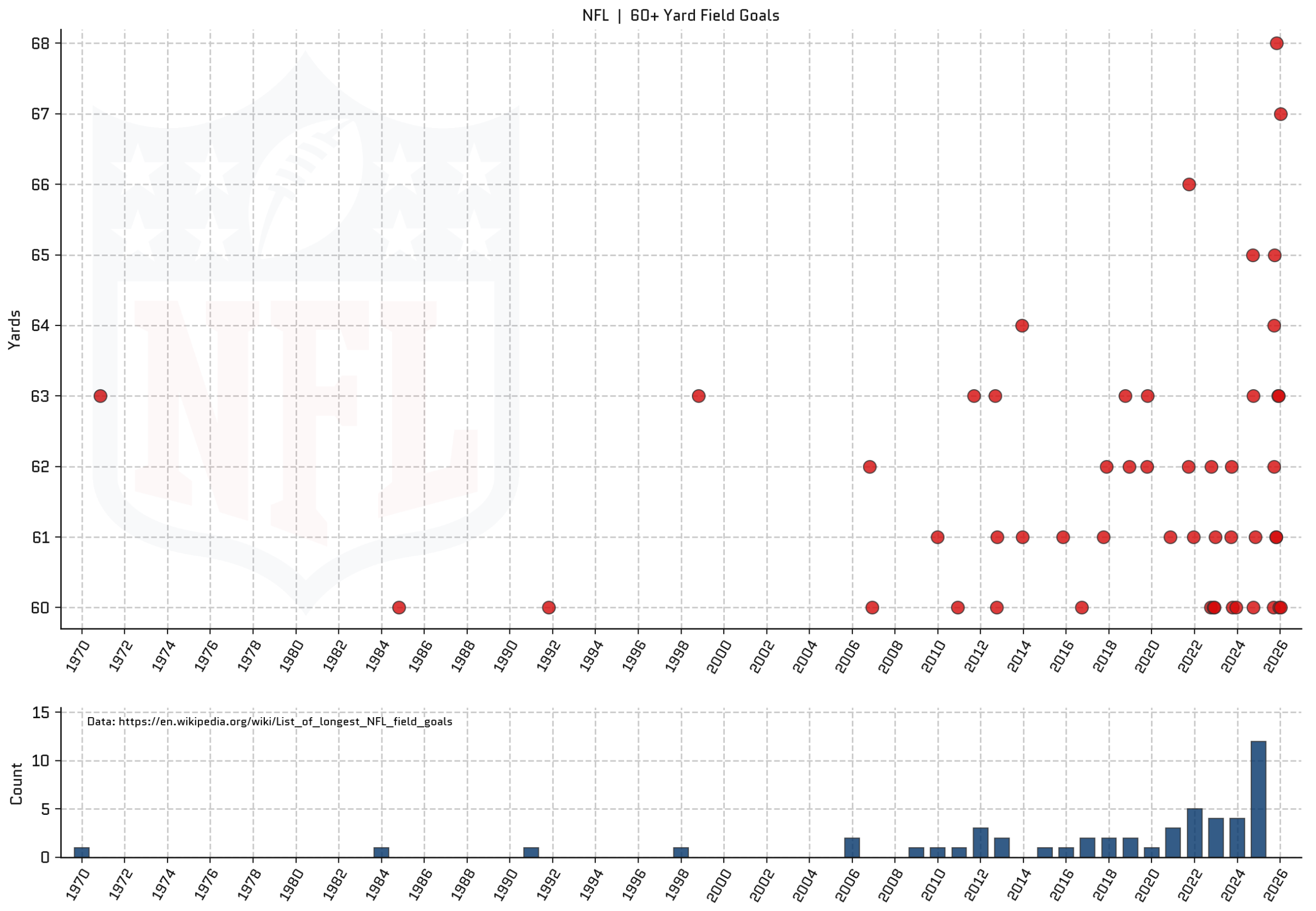
I like the dashed grid lines. They aren’t something I usually go for but they somehow remind me of football field markings.
We can see that 60+ yard field goals started becoming more common in the late 2000s and took off beginning in 2021. Then 2025 was a total blowout, tripling the previous year.
And it wasn’t just one guy making all these kicks. Cam Little set the NFL record of 68 yards but 9 different kickers contributed to the total of 12 last year.
Maybe there will be some mean reversion this upcoming season and we’ll only see half as many bombs. Even then, no one could deny we’ve entered a golden age of field goal kicking. Enjoy it while it lasts.
Full code:
scrape_data.py
import requests
from io import StringIO
import pandas as pd


url = "https://en.wikipedia.org/wiki/List_of_longest_NFL_field_goals"

headers = {"User-Agent": "KickerBot/1.0"}

text = requests.get(url, headers=headers).text

with open("response.txt", "w") as f:
    f.write(text)

with open("response.txt", "r") as f:
    text = f.read()

dfs_found = pd.read_html(StringIO(text))

df = dfs_found[0][['Distance', 'Date', 'Kicker']].copy()

df['Date'] = pd.to_datetime(df['Date'])

df['Distance'] = df['Distance'].str.strip(" yards").astype(int)

df.to_csv("nfl_fgs_2026-09-03.csv", index=False)
plot_data.py
import pandas as pd
import matplotlib.pyplot as plt
from matplotlib.offsetbox import OffsetImage, AnnotationBbox


df = pd.read_csv("nfl_fgs_2026-09-03.csv", parse_dates=['Date'])

df['Season'] = (df['Date'] - pd.Timedelta("90 days")).dt.strftime("%Y").astype(int)

df['Season_x'] = df['Season'].apply(lambda x: pd.Timestamp(f"January 1 {x}"))

df2 = df.groupby("Season_x")['Distance'].agg("count").reset_index()

plt.style.use("wollen_nfl.mplstyle")

fig, (ax0, ax1) = plt.subplots(nrows=2,
                               ncols=1,
                               height_ratios=(4, 1))

edge_color = "#333"
edge_width = 0.8
alpha = 0.8

ax0.scatter(df['Date'],
            df['Distance'],
            color="#D50A0A",
            edgecolor=edge_color,
            linewidth=edge_width,
            alpha=alpha)

ax1.bar(df2['Season_x'],
        df2['Distance'],
        width=250,
        color="#013369",
        edgecolor=edge_color,
        linewidth=edge_width,
        alpha=alpha)

x_ticks = pd.date_range(start="1970",
                        end="2026",
                        freq="2YS")

x_tick_labels = [item.strftime("%Y") for item in x_ticks]

x_limits = (pd.Timestamp("Jan 1 1969"), pd.Timestamp("Jan 1 2027"))

ax0.set(xticks=x_ticks,
        xticklabels=x_tick_labels,
        xlim=x_limits,
        yticks=range(60, 69),
        ylim=(59.7, 68.2),
        ylabel="Yards",
        title="NFL  |  60+ Yard Field Goals")

ax1.set(xticks=x_ticks,
        xticklabels=x_tick_labels,
        xlim=x_limits,
        yticks=range(0, 20, 5),
        ylim=(0, 15.5),
        ylabel="Count")

for ax in [ax0, ax1]:
    plt.setp(ax.xaxis.get_majorticklabels(),
             rotation=60,
             horizontalalignment="right",
             rotation_mode="anchor")

ax1.text(x=pd.Timestamp("April 1 1970"),
         y=14.5,
         s="Data: https://en.wikipedia.org/wiki/List_of_longest_NFL_field_goals",
         size=8,
         horizontalalignment="left",
         verticalalignment="top",
         bbox={"facecolor": "white", "edgecolor": "None", "pad": 0})

ab = AnnotationBbox(OffsetImage(plt.imread("nfl_logo.png"),
                                zoom=0.27,
                                alpha=0.03),
                    xy=(pd.Timestamp("July 1 1970"), 67.9),
                    box_alignment=(0, 1),
                    frameon=False)

ax0.add_artist(ab)

plt.savefig("nfl_field_goals.png", dpi=200)